ptonsparky
Tom
- Occupation
- EC - retired
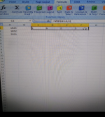
1625 | |||||
1 | 6 | 2 | 5 |
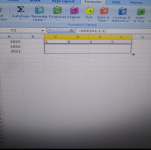
1625 | |||||
1 | 6 | 2 | 5 |

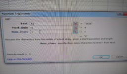
Truncate was the function I was looking for, but that by itself isn't workingTom, here is one way to separate your original 1632 into separate digits using formulas...
View attachment 2569750
Your original number is in cell B40.
To get the "1" digit - the formula I used is =TRUNC(B40/1000)
This divides 1632 by 1000 to get 1.632. The Truncate function eliminates the decimal portion (.632), leaving the "1"
To get the next digit ("6"), you do something similar. That formula is =TRUNC(B40/100) - (C40*10)
This divides 1632 by 100 to get 16.32. Then truncate it to leave 16. Then subtracts the answer from C40 (the "1") times 10
1632/100 -> 16.32 -> 16 -> subtract the 10 leaves 6
Same ideas for the "3" and the "2". It just keeps getting one calculation longer each time. For the "3", you have to subtract 100 and 60 from 163.
For the "2" you don't need to truncate anymore, you simply subtract 1000, and 600 and 30 from your original 1632
Not sure if this helps any.
That works one time. The process needs to be repeated each time the value is changed.“Data—>Text to columns”.
This starts a parsing wizard that’s simple to use.
Does the formula approach I posted above help? You say the TRUNC function is not working by itself. Not quite sure what you mean by that.Truncate was the function I was looking for, but that by itself isn't working
Yes, got it to work for the range of 1100 to 9900 but not for outside of that range. IIRC. My memory is as short as my small digit. Makes my eyes cross thinking of what I need to do for 99 mega ohm.Does the formula approach I posted above help? You say the TRUNC function is not working by itself. Not quite sure what you mean by that.
Did you see the formulas I used for cells C40, D40, E40 and F40 in my post above.
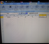
Oooh, I like that! Much more straightforward than my formulas.Use the MID function.
None of the examples so far really do what you want.What I want to do is separate the number into color codes for a resistor. 1st,, 2nd, and multiplier for a 4 band.
1600 would be a better #. (1, 6, 100)
Pretty sure what I supplied is what he ask for. He ask for a way to take the four digit number and put each in it's own cell in order.None of the examples so far really do what you want.
can you give more examples of the numbers your using?
Thats what my post #2 does without formulas Using data tab and text to columns.Pretty sure what I supplied is what he ask for. He ask for a way to take the four digit number and put each in it's own cell in order.
From there he can assign a multiplier function.
Agreed it may be what he want as a end result.
You are correct, sorry and thank youThats what my post #2 does without formulas Using data tab and text to columns.
in post #3, last sentence he's asking for something different.
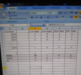
| Insert known values @ RED text | |||||||||
| Known Value | 1120 | =MID($B$2,1,1) | =MID($B$2,2,1) | =MID($B$2,3,1) | =MID($B$2,4,1) | =MID($B$2,5,1) | =MID($B$2,6,1) | =MID($B$2,7,1) | =MID($B$2,8,1) |
| Multiplier if Above is <1000 | 0.01 | =C2*1 | =D2*1 | =E2*1 | |||||
| Tolerance | 0.1 | =VLOOKUP(C3,D14:E23,2,1) | =VLOOKUP(D3,D14:E23,2,1) | =VLOOKUP(E3,D14:E23,2,1) | =VLOOKUP(H4,J12:L23,3,2) | =VLOOKUP(B4,A14:B18,2,1) | =IF(I4>0,I4,B3) | =COUNTIF(F2:O2,0) | |
| Band | 1st | 2nd | 3rd | 4th Multiplier | 5th Tolerance | ||||
| Insert known values @ RED text | |||||||||
| Known Value | 1120 | 1 | 1 | 2 | 0 | ||||
| Multiplier if Above is <1000 | 0.01 | 1 | 1 | 2 | |||||
| Tolerance | 0.1 | BROWN | BROWN | RED | BLACK | SILVER | 1 | 1 | |
| Band | 1st | 2nd | 3rd | 4th Multiplier | 5th Tolerance | ||||